Accessing the GMF components

In this tutorial, we show how to access the different magnetic field components of the models of the Galactic magnetic field from Jansson & Farrar (2012), Pshirkov et al. (2011) and Unger & Farrar (2024).

We begin with the necessary imports and defining a grid in galacto-centric coordinates.

[1]:

from gammaALPs.bfields import gmf
import numpy as np
import matplotlib.pyplot as plt
from matplotlib.colors import LinearSegmentedColormap
from matplotlib.colors import TwoSlopeNorm

fatal: No names found, cannot describe anything.

First we build 3D coordinate arrays in galactocentric cartesian (\(x, y, z\)) and cylindrical coordinates \((\rho, \phi, z)\), where \(x, y, z\) and \(\rho\) are in units of kpc.

[2]:

x = np.linspace(-20.,20.,300)
y = np.linspace(-20.,20.,300)
z = np.arange(-5.,5.01,0.01)
xx, yy, zz = np.meshgrid(x, y, z, indexing = 'ij')

rr = np.sqrt(xx ** 2. + yy ** 2.) # rho component
pp = np.arctan2(yy, xx) # phi component

The Pshirkov model

For the Pshirkov model, both the bisymmetric (BSS) and the axisymmetric (ASS) versions are available. We illustrate the model and its usage for the ASS version.

The model is simply initialized like this:

[3]:

pshirkov = gmf.GMFPshirkov(model='ASS')

The model has two \(B\)-field components: the field in the halo and in the disk. To show the disk component, we select the \(z\) component that is closest to \(z=0\):

[4]:

idz = np.argmin(np.abs(z))

Then we calculate and plot the disk component through the Bdisk function. We multiply the abolute value of the field with the gmf.signum function to determine the sign of the \(B\)-field relative to the \(z=0\) plane.

[5]:

Bdisk = np.zeros_like(rr[...,idz])

for i, r in enumerate(rr[...,idz]):
    # returns (3,N),(N) tuple, first entry is field, second entry is absolute value
    b = pshirkov.Bdisk(rho=r, phi=pp[:,i,idz], z=zz[:,i,idz])
    Bdisk[:,i] = b[1] * gmf.signum(b[0][1,:])

And plot the results:

[6]:

im = plt.pcolormesh(xx[...,idz], yy[...,idz], Bdisk, cmap=plt.cm.RdBu_r, shading='auto')
plt.xlabel('x (kpc)')
plt.ylabel('y (kpc)')
plt.colorbar(im, label = '$B (\mu\mathrm{G})$')

[6]:

<matplotlib.colorbar.Colorbar at 0x7fd9e60e26e0>

../_images/tutorials_accessing_GMF_components_13_1.png

We proceed similarly for the halo component by finding the index where \(y = 0\) (or closest to it):

[7]:

idy = np.argmin(np.abs(y))

And calculate the halo component in the same way as the disk component:

[8]:

Bhalo = np.zeros_like(xx[:,idy,:])
for i,xi in enumerate(xx[:,idy,:]):
    # returns (3,N),(N) tuple, first entry is field, second entry is abs value
    b = pshirkov.Bhalo(rho=np.sqrt(xi**2. + y[idy]**2.),
                       z=zz[i,idy,:])
    Bhalo[i,:] = b[1]

[9]:

im = plt.pcolormesh(xx[:,idy,:], zz[:,idy,:], Bhalo, cmap=plt.cm.RdBu_r, shading='auto')
plt.xlabel('x (kpc)')
plt.ylabel('z (kpc)')
plt.colorbar(im, label = '$B (\mu\mathrm{G})$')

[9]:

<matplotlib.colorbar.Colorbar at 0x7fd9e3bd5780>

../_images/tutorials_accessing_GMF_components_18_1.png

The total magnetic field would then be found by summing the Bdisk and Bhalo vectors (evaluated over the same coordinate grid).

The Jansson & Farrar model

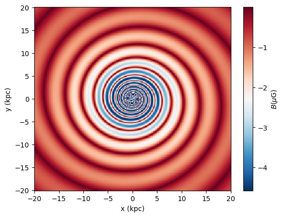
We follow the same steps for the Jansson & Farrar model. The only difference here is that this model has an additional “X” component which we will plot as well.

We initiate the class like this:

[10]:

jansson = gmf.GMF()

Print the magnetic field in the 8th ring, which is given by \(b_8 = \sum_{i=1}^7 b_i f_i / f_8\), where the \(f_i\) is relative cross-sectional areas of the spirals (for a fixed radius) and \(b_i\) is the mangetic field in each spiral arm (see Jansson & Farrar (2012), Sec. 5.1.1).

[11]:

print (jansson.b[7])

2.755128205128205

Now calculate the disk component:

[12]:

Bdisk = np.zeros_like(rr[...,idz])
for i,r in enumerate(rr[...,idz]):
    b = jansson.Bdisk(rho=r, phi=pp[:,i,idz], z=zz[:,i,idz])
    Bdisk[:,i] = b[1] * gmf.signum(b[0][1,:])

And for some specific positions, at which we want to place arrows in the plot

[13]:

# position of arrows in plot
rho0 = np.array([4., 5.5, 6.5, 8., 9., 10.5, 12, 16.5])
phi0 = np.array([5. * np.pi / 4.])

Bdisk_arrow = np.zeros([3, rho0.size])
for i, r in enumerate(rho0):
    b = jansson.Bdisk(np.array([r]), phi0, z=z[idz])[0]
    Bdisk_arrow[:,i] = b[:,0]

# now transform Bdisk_arrow components (rho, phi, z)
# to cartesian coordinates
Bdisk_x = np.zeros_like(Bdisk_arrow)  # disk component in cartesian coordinates
Bdisk_x[0] = np.cos(phi0) * Bdisk_arrow[0] - np.sin(phi0) * Bdisk_arrow[1]
Bdisk_x[1] = np.sin(phi0) * Bdisk_arrow[0] + np.cos(phi0) * Bdisk_arrow[1]
Bdisk_x[2] = Bdisk_arrow[2]

Plotting it:

[14]:

im = plt.pcolormesh(xx[...,idz], yy[...,idz], Bdisk, cmap=plt.cm.RdBu_r, shading='auto')

# the arrows
plt.quiver(rho0 * np.cos(phi0), rho0 * np.sin(phi0),
           Bdisk_x[0] / np.sqrt(np.sum(Bdisk_x**2., axis = 0)),
           Bdisk_x[1] / np.sqrt(np.sum(Bdisk_x**2., axis = 0)),
          )

plt.xlabel('x (kpc)')
plt.ylabel('y (kpc)')
plt.colorbar(im, label = '$B (\mu\mathrm{G})$')

[14]:

<matplotlib.colorbar.Colorbar at 0x7fd9e5ea7340>

../_images/tutorials_accessing_GMF_components_29_1.png

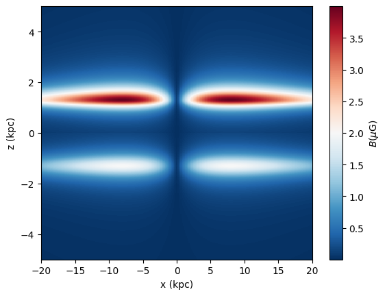
Proceeding with the halo component in the same way as before:

[15]:

Bhalo = np.zeros_like(xx[:,idy,:])
for i,xi in enumerate(xx[:,idy,:]):
    b = jansson.Bhalo(rho=np.sqrt(xi**2. + y[idy]**2.),
                       z=zz[i,idy,:])
    Bhalo[i,:] = b[1]

[16]:

im = plt.pcolormesh(xx[:,idy,:], zz[:,idy,:], Bhalo, cmap=plt.cm.RdBu_r, shading='auto')
plt.xlabel('x (kpc)')
plt.ylabel('z (kpc)')
plt.colorbar(im, label = '$B (\mu\mathrm{G})$')

[16]:

<matplotlib.colorbar.Colorbar at 0x7fd9e5da2c80>

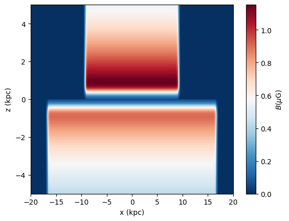
../_images/tutorials_accessing_GMF_components_32_1.png

And the additional “X” component:

[17]:

BX_abs = np.zeros_like(xx[:,idy,:])
BX = np.zeros([3] + list(xx[:,idy,:].shape))

for i,xi in enumerate(xx[:,idy,:]):
    b = jansson.BX(rho=np.sqrt(xi**2. + y[idy]**2.),
                       z=zz[i,idy,:])
    BX_abs[i,:] = b[1]
    BX[:, i, :] = b[0]

# now transform Bdisk_arrow components (rho, phi, z)
# to cartesian coordinates
# note that phi component is zero
BX_x = BX[0] * np.cos(pp[:,idy,...])
BX_y = BX[0] * np.sin(pp[:,idy,...])

BX_z = BX[2]

[18]:

p = plt.pcolormesh(xx[:,idy,:], zz[:,idy,:], BX_abs, cmap=plt.cm.RdBu_r, shading='auto')

# plot the arrows
# at z = 0
idz = int(len(z) / 2)
step = 4
plt.quiver(xx[:,idy,idz][::step],  zz[:,idy,idz][::step],
           BX_x[:,idz][::step] / BX_abs[:,idz][::step], BX_z[:,idz][::step] / BX_abs[:,idz][::step],
           width=3e-3, scale=25
          )

# arrows below disk
idz = int(len(z) / 2) - 70
plt.quiver(xx[:,idy,idz][::step],  zz[:,idy,idz][::step],
           BX_x[:,idz][::step] / BX_abs[:,idz][::step], BX_z[:,idz][::step] / BX_abs[:,idz][::step],
           width=3e-3, scale=25
          )

plt.xlabel('x (kpc)')
plt.ylabel('z (kpc)')
plt.colorbar(p, label = '$B (\mu\mathrm{G})$')

/tmp/ipykernel_209855/2324834406.py:8: RuntimeWarning: invalid value encountered in divide
  BX_x[:,idz][::step] / BX_abs[:,idz][::step], BX_z[:,idz][::step] / BX_abs[:,idz][::step],
/tmp/ipykernel_209855/2324834406.py:15: RuntimeWarning: invalid value encountered in divide
  BX_x[:,idz][::step] / BX_abs[:,idz][::step], BX_z[:,idz][::step] / BX_abs[:,idz][::step],

[18]:

<matplotlib.colorbar.Colorbar at 0x7fd9e611ae90>

../_images/tutorials_accessing_GMF_components_35_2.png

Again, the total magnetic field would be found by summing the Bdisk, Bhalo, and BX vectors evaluated over the same coordinate grid.

The Unger & Farrar model (UF23)

The UF23 Model consists of a set of eight models that can be constructed with five different components. The different components can be accessed similarly to the Pshirkov and JF12 model.

[19]:

models = ['base', 'expX', 'neCL', 'twistX', 'nebCor', 'cre10', 'synCG', 'spur']

[20]:

x = np.linspace(-20.,20.,200)
y = np.linspace(-20.,20.,200)
z = np.arange(-5.,5.01,0.05)
xx, yy, zz = np.meshgrid(x, y, z, indexing = 'ij')

rr = np.sqrt(xx ** 2. + yy ** 2.) # rho component
pp = np.arctan2(yy, xx) # phi component

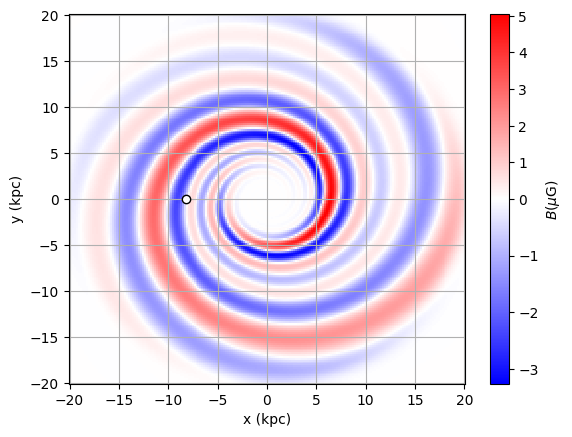
For the disk field there are two components implemented. The grand fourier spiral is used in 7 of the 8 models (we use the “base” model as example) and the spiral spur field is used in the “spur” model.

Fourier Spiral

We initialize the class for the ‘base’ model:

[21]:

uf23 = gmf.UF23(model='base')

We calculate the \(B\)-Field at \(z = 0\)

[22]:

zplot = 0
idz = np.absolute(z-zplot).argmin()

Now we calculate the fourier-spiral disk field

[23]:

Bdisk = np.zeros_like(rr[...,idz])
for i,r in enumerate(rr[...,idz]):
    # returns (3,N),(N) tuple, first entry is field vector, second entry is abs value
    b = uf23.Bdisk(rho=r, phi=pp[:,i,idz], z=zz[:,i,idz])
    # same as uf23.spiral_field(...)
    Bdisk[:,i] = b[1] * gmf.signum(b[0][1,:])

Instead of uf23.Bdisk(), we could also use uf23.spiral_field(). Bdisk() just chooses between spiral_field() and spur_field() depending on the chosen model.

Plotting:

[24]:

norm = TwoSlopeNorm(vmin=Bdisk.min(), vcenter=0, vmax=Bdisk.max())
p = plt.pcolormesh(xx[...,idz], yy[...,idz], Bdisk, norm=norm, cmap = plt.cm.bwr, shading='auto')

plt.xlabel('x (kpc)')
plt.ylabel('y (kpc)')
plt.colorbar(p, label = '$B (\mu\mathrm{G})$')

# position of sun
plt.plot(-8.2, 0., marker='o', mec='k', mfc='w')
plt.grid()

plt.show()

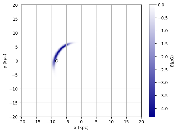
../_images/tutorials_accessing_GMF_components_51_0.png

Spiral Spur

The spiral spur component is only used in the “spur” model. So we initialize the class with the other model and calculate again the disk field using the same function as above.

[25]:

spur = gmf.UF23(model='spur')

[26]:

Bdisk_spur = np.zeros_like(rr[...,idz])
for i,r in enumerate(rr[...,idz]):
    # returns (3,N),(N) tuple, first entry is field, second entry is abs value
    b = spur.Bdisk(rho=r, phi=pp[:,i,idz], z=zz[:,i,idz])
    # same as spur.spiral_spur(...)
    Bdisk_spur[:,i] = b[1] * gmf.signum(b[0][1,:])

[27]:

cmap0 = LinearSegmentedColormap.from_list('', ['darkblue', 'white'])

p = plt.pcolormesh(xx[...,idz], yy[...,idz], Bdisk_spur, cmap = cmap0, shading='auto')

plt.xlabel('x (kpc)')
plt.ylabel('y (kpc)')
plt.colorbar(p, label = '$B (\mu\mathrm{G})$')

# position of sun
plt.plot(-8.2, 0., marker='o', mec='k', mfc='w')
plt.grid()

plt.show()

../_images/tutorials_accessing_GMF_components_56_0.png

Halo Field

For the Halo field there are three components implemented: toroidal_halo_field(), poloidal_halo_field(), and twisted_halo_field(). Seven of the 8 models use the sum of the toroidal and poloidal halo field, and the “twistX” model uses the twisted_halo_field(). The function Bhalo() would return either the sum of toroidal and poloidal halo field or the twisted halo field depending on the chosen model.

The components can also be accessed seperately:

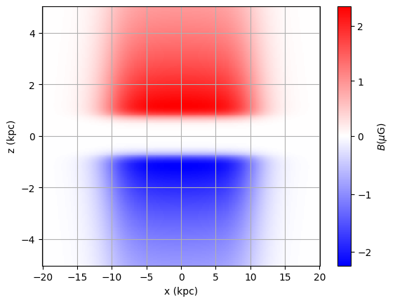
Toroidal Halo

We calculate the toroidal halo in the \(x\)-\(z\)-plane at \(y=0\)

[28]:

yplot = 0
idy = np.absolute(y-yplot).argmin()

We use again the “base” model for example and do a similar calculation:

[29]:

Bhalo_tor = np.zeros_like(xx[:,idy,:])
for i,xi in enumerate(xx[:,idy,:]):
    # returns (3,N),(N) tuple, first entry is field, second entry is abs value
    b = uf23.toroidal_halo_field(rho=np.sqrt(xi**2. + y[idy]**2.), z=zz[i,idy,:])
    Bhalo_tor[i,:] = b[1] * gmf.signum(b[0][1,:])

[30]:

norm = TwoSlopeNorm(vmin=Bhalo_tor.min(), vcenter=0, vmax=Bhalo_tor.max())
p = plt.pcolormesh(xx[:,idy,:], zz[:,idy,:], Bhalo_tor, norm=norm, cmap = plt.cm.bwr, shading='auto')

plt.xlabel('x (kpc)')
plt.ylabel('z (kpc)')
plt.colorbar(p, label = '$B (\mu\mathrm{G})$')

plt.grid()

plt.show()

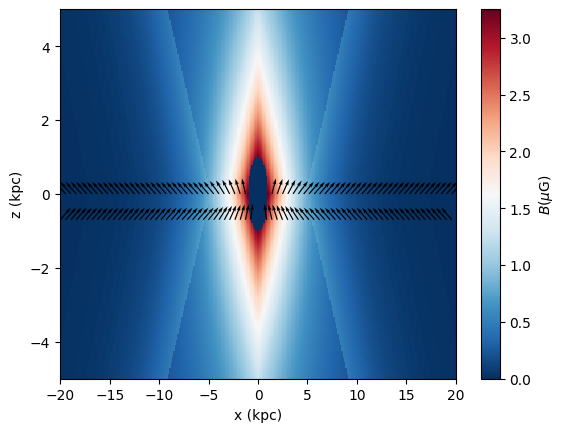
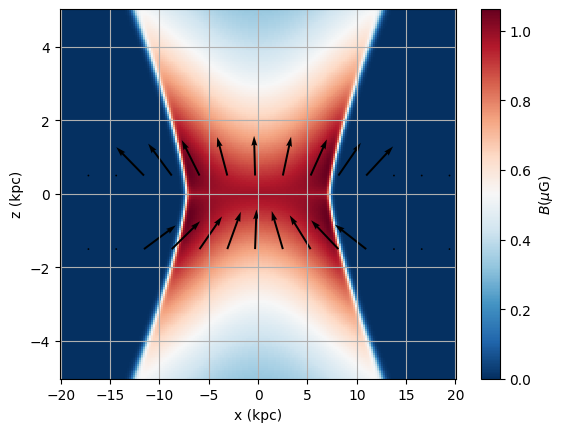
../_images/tutorials_accessing_GMF_components_65_0.png

Poloidal Halo

Additionally to the torodial halo field, the UF23 model contains a poloidal halo component, similar to the X-Field in the JF12 model. The poloidal component has two functions for the radial dependence, depending on the chosen model. For the “expX” model a exponential function is used, while the other models use a sigmoid function. For the “base” model we get:

[31]:

BX = np.zeros([3] + list(xx[:,idy,:].shape))
BX_abs = np.zeros_like(xx[:,idy,:])
for i,xi in enumerate(xx[:,idy,:]):
    b = uf23.poloidal_halo_field(rho=np.sqrt(xi**2. + y[idy]**2.),
                       z=zz[i,idy,:])
    BX_abs[i,:] = b[1]
    BX[:, i, :] = b[0]

# convert to cartesian coordinates, phi component is zero
BX_x = BX[0] * np.cos(pp[:,idy,...])
BX_y = BX[0] * np.sin(pp[:,idy,...])
BX_z = BX[2]
BX_abss = np.where(BX_abs == 0, 1e-24, BX_abs)

Plot with arrows:

[32]:

cmap0 = LinearSegmentedColormap.from_list('', ['white', 'red'])

p = plt.pcolormesh(xx[:,idy,:], zz[:,idy,:], BX_abs, cmap=plt.cm.RdBu_r, shading='auto')

plt.colorbar(p, label = '$B (\mu\mathrm{G})$')

z0 = 0.5
idz = np.absolute(z-z0).argmin()

step = 14
plt.quiver(xx[:,idy,idz][::step],  zz[:,idy,idz][::step],
           BX_x[:,idz][::step] / BX_abss[:,idz][::step], BX_z[:,idz][::step] / BX_abss[:,idz][::step],
           width=5e-3, scale=10
          )

z0 = -1.5
idz = np.absolute(z-z0).argmin()

plt.quiver(xx[:,idy,idz][::step],  zz[:,idy,idz][::step],
           BX_x[:,idz][::step] / BX_abss[:,idz][::step], BX_z[:,idz][::step] / BX_abss[:,idz][::step],
           width=5e-3, scale=10
          )

plt.xlabel('x (kpc)')
plt.ylabel('z (kpc)')
plt.grid()

plt.show()

../_images/tutorials_accessing_GMF_components_70_0.png

Twisted Halo Field

Instead of a seperate poloidal and toroidal halo field, the “twistX” model uses a unified halo, the twisted_halo_field() component. It can be accessed by initializing the UF23 class with the UF23 model:

[33]:

twisted = gmf.UF23(model='twistX')

and then using either twisted.Bhalo(), or twisted.twisted_halo_field().

The total magnetic field is always given through uf23.Bdisk()[0] + uf23.Bhalo()[0]. Depending on the chosen model, the right components are selected and summed up.