![]()
Photon-photon dispersion
This tutorial shows how to include photon-photon dispersion off of background photon fields in the ALP-photon propagation calculation. The relevance of photon dispersion for ALP calculations is discussed in Dobrynina 2015. A background field adds to the dispersive part of the refractive index of the propagation medium \(n = 1+\chi\). Dobrynina 2015 show that at \(z=0\), \(\chi_{CMB} = 5.11\times10^{-43}\). Dispersion off the CMB is included by default, but other values of \(\chi\) can be included manually.
If you haven’t installed gammaALPs already, you can do so using pip. Just uncomment the line below:
[1]:
#!pip install gammaALPs
First import what we will need:
[2]:
from gammaALPs.core import Source, ALP, ModuleList
from gammaALPs.base import environs, transfer
import numpy as np
import matplotlib.pyplot as plt
from astropy import constants as c
from matplotlib.patheffects import withStroke
from astropy import units as u
import time
from scipy.interpolate import RectBivariateSpline as RBSpline

effect  = dict(path_effects=[withStroke(foreground="w", linewidth=2)])  # used for plotting
\(\chi\) is included in the code as a 2D spline function in energy and propagation distance. This means that the points at which \(\chi\) is calculated at do not need to be exactly the same as the points used for the magnetic field. It is also possible to include \(\chi\) as an array of size (1) if you want a constant value, or size (len(EGeV),len(r)), if you have calculated \(\chi\) in the exact magnetic field domains you will be using.
\(\chi\) function
We will create a fake \(\chi\) function which changes with distance and energy, and then see its effects on mixing in different environments.
[3]:
EGeV = np.logspace(-5.,6.,1000)
[4]:
chiCMB = transfer.chiCMB
[5]:
chiCMB
[5]:
5.0962922355799666e-43
\(r\) will be in pc for the jets and kpc for the clusters and GMF.
[6]:
rs = np.logspace(-2,5,200)
chis = 1.e9 * rs[np.newaxis,:]**-3 * chiCMB * EGeV[:,np.newaxis]**(1.5) + chiCMB
[7]:
plt.loglog(rs,chis[0,:])
plt.loglog(rs,chis[500,:])
plt.loglog(rs,chis[-1,:])
plt.ylabel(r'$\chi$')
plt.xlabel('r [pc or kpc] or z')
[7]:
Text(0.5, 0, 'r [pc or kpc] or z')
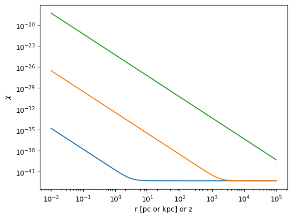
Our \(\chi\) changes with both energy and distance.
[8]:
ee, rr = np.meshgrid(EGeV,rs,indexing='ij')
plt.pcolormesh(ee,rr,np.log10(chis),cmap=plt.get_cmap('coolwarm'),
               shading='auto')
plt.colorbar(label=r"log($\chi$)")
plt.xscale('log')
plt.yscale('log')
plt.xlabel('E [GeV]')
plt.ylabel('r [pc or kpc]')
[8]:
Text(0, 0.5, 'r [pc or kpc]')
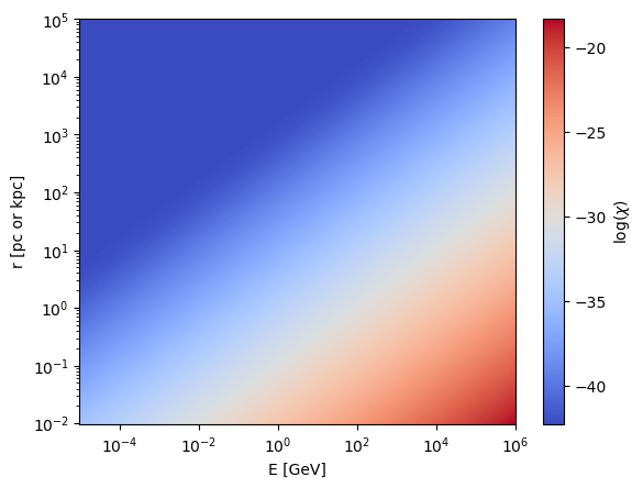
Make the spline function:
[9]:
chispl = RBSpline(EGeV,rs,chis,kx=1,ky=1,s=0)
Now we can test it for a source. We will use 3C454.3 (see the individual environment tutorials for more details on each of the environments).
[10]:
src = Source(z=0.859 , ra='22h53m57.7s', dec='+16d08m54s', bLorentz=60.) # 3C454.3
[11]:
pin = np.diag((1.,1.,0.)) * 0.5
Jet
First, let’s test the "Jet" class:
[12]:
ml = ModuleList(ALP(m=1., g=2.), src, pin=pin, EGeV=EGeV, seed = 0)
ml_chi = ModuleList(ALP(m=1., g=2.), src, pin=pin, EGeV=EGeV, seed = 0)
[13]:
# other jet
gamma_min = 18.
Add the same jet module to each, including \(\chi\) with the chi keyword for the second one.
[14]:
ml.add_propagation("Jet",
                  0,  # position of module counted from the source.
                  B0=0.32,  # Jet field at r = R0 in G
                  r0=1.,  # distance from BH where B = B0 in pc
                  rgam=3.19e17 * u.cm.to('pc'),  # distance of gamma-ray emitting region to BH
                  alpha=-1.,  # exponent of toroidal mangetic field (default: -1.)
                  psi=np.pi/4.,  # Angle between one photon polarization state and B field.
                                 # Assumed constant over entire jet.
                  helical=True,  # if True, use helical magnetic-field model from Clausen-Brown et al. (2011).
                                 # In this case, the psi kwarg is treated is as the phi angle
                                 # of the photon trajectory in the cylindrical jet coordinate system
                  equipartition=True,  # if true, assume equipartition between electrons and the B field.
                                       # This will overwrite the exponent of electron density beta = 2 * alpha
                                       # and set n0 given the minimum electron lorentz factor set with gamma_min
                  gamma_min=gamma_min,  # minimum lorentz factor of emitting electrons, only used if equipartition=True
                  gamma_max=np.exp(10.) * gamma_min,  # maximum lorentz factor of emitting electrons,
                                                      # only used if equipartition=True
                  Rjet= 40.,  # maximum jet length in pc (default: 1000.)
                  n0=1e4,  # normalization of electron density, overwritten if equipartition=True
                  beta=-2.    # power-law index of electron density, overwritten if equipartition=True
                 )
ml_chi.add_propagation("Jet",
                  0,  # position of module counted from the source.
                  B0=0.32,  # Jet field at r = R0 in G
                  r0=1.,  # distance from BH where B = B0 in pc
                  rgam=3.19e17 * u.cm.to('pc'),  # distance of gamma-ray emitting region to BH
                  alpha=-1.,  # exponent of toroidal mangetic field (default: -1.)
                  psi=np.pi/4.,  # Angle between one photon polarization state and B field.
                                 # Assumed constant over entire jet.
                  helical=True,  # if True, use helical magnetic-field model from Clausen-Brown et al. (2011).
                                 # In this case, the psi kwarg is treated is as the phi angle
                                 # of the photon trajectory in the cylindrical jet coordinate system
                  equipartition=True,  # if true, assume equipartition between electrons and the B field.
                                       # This will overwrite the exponent of electron density beta = 2 * alpha
                                       # and set n0 given the minimum electron lorentz factor set with gamma_min
                  gamma_min=gamma_min,  # minimum lorentz factor of emitting electrons, only used if equipartition=True
                  gamma_max=np.exp(10.) * gamma_min,  # maximum lorentz factor of emitting electrons,
                                                      # only used if equipartition=True
                  Rjet= 40.,  # maximum jet length in pc (default: 1000.)
                  n0=1e4,  # normalization of electron density, overwritten if equipartition=True
                  beta=-2.,    # power-law index of electron density, overwritten if equipartition=True
                  chi=chispl
                 )
environs.py: 758 --- INFO: Assuming equipartion at r0: n0(r0) = 6.307e-01 cm^-3
environs.py: 767 --- INFO: Using inputted chi
environs.py: 758 --- INFO: Assuming equipartion at r0: n0(r0) = 6.307e-01 cm^-3
environs.py: 764 --- INFO: Using interpolated chi
Pick a mass and coupling where there is some mixing, and run the calculation for each.
[15]:
ml.alp.m = 100.
ml.alp.g = 0.3

ml_chi.alp.m = 100.
ml_chi.alp.g = 0.3
[16]:
px, py, pa = ml.run()
pgg = px + py

px_c, py_c, pa_c = ml_chi.run()
pgg_chi = px_c + py_c
   core.py: 658 --- INFO: Running Module 0: <class 'gammaALPs.base.environs.MixJet'>
/Users/mey/Python/gammaALPs/gammaALPs/base/transfer.py:799: UserWarning: Not all values of linear polarization are real values!
  warnings.warn("Not all values of linear polarization are real values!")
/Users/mey/Python/gammaALPs/gammaALPs/base/transfer.py:802: UserWarning: Not all values of circular polarization are real values!
  warnings.warn("Not all values of circular polarization are real values!")
   core.py: 658 --- INFO: Running Module 0: <class 'gammaALPs.base.environs.MixJet'>
[17]:
for p in pgg:
    plt.plot(ml.EGeV, p, label=r'$\chi_{CMB}$')

for p_c in pgg_chi:
    plt.plot(ml_chi.EGeV, p_c, label=r'$\chi$-spline')

plt.grid(True, lw = 0.2)
plt.grid(True, which = 'minor', axis = 'y', lw = 0.2)

plt.xlabel('Energy (GeV)')
plt.ylabel(r'Photon survival probability')

plt.gca().set_xscale('log')
plt.annotate(r'$m_a = {0:.1f}\,\mathrm{{neV}}, g_{{a\gamma}}'
             r' = {1:.2f} \times 10^{{-11}}\,\mathrm{{GeV}}^{{-1}}$'.format(ml.alp.m,ml.alp.g),
             xy=(0.05,0.1),
             size='large',
             xycoords='axes fraction',
             ha='left',
             **effect)
plt.legend(loc='upper left')
[17]:
<matplotlib.legend.Legend at 0x145ef8cd0>
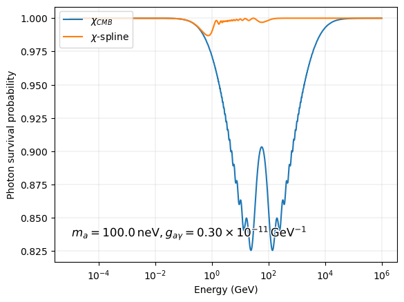
The \(P_{\gamma\gamma}\)’s are quite different between the two cases. \(\chi\) affects the mixing by lowering the high critical energy, \(E_{crit}^{high}\), and so oftern reduces mixing at very high energies.
Cluster
Now let’s look at a cluster magnetic field, "ICMGaussTurb". We can use the same \(\chi\) array in \((E,r)\) but this time \(r\) will be in kpc instead of pc.
[18]:
# cluster
ml = ModuleList(ALP(m=1., g=2.), src, pin=pin, EGeV=EGeV, seed = 0)
ml_chi = ModuleList(ALP(m=1., g=2.), src, pin=pin, EGeV=EGeV, seed = 0)
[19]:
ml.add_propagation("ICMGaussTurb",
                  0, # position of module counted from the source.
                  nsim=1, # number of random B-field realizations
                  B0=10.,  # rms of B field
                  n0=39.,  # normalization of electron density
                  n2=4.05, # second normalization of electron density, see Churazov et al. 2003, Eq. 4
                  r_abell=500., # extension of the cluster
                  r_core=80.,   # electron density parameter, see Churazov et al. 2003, Eq. 4
                  r_core2=280., # electron density parameter, see Churazov et al. 2003, Eq. 4
                  beta=1.2,  # electron density parameter, see Churazov et al. 2003, Eq. 4
                  beta2=0.58, # electron density parameter, see Churazov et al. 2003, Eq. 4
                  eta=0.5, # scaling of B-field with electron denstiy
                  kL=0.18, # maximum turbulence scale in kpc^-1, taken from A2199 cool-core cluster, see Vacca et al. 2012
                  kH=9.,  # minimum turbulence scale, taken from A2199 cool-core cluster, see Vacca et al. 2012
                  q=-2.80, # turbulence spectral index, taken from A2199 cool-core cluster, see Vacca et al. 2012
                  seed=0 # random seed for reproducability, set to None for random seed.
                 )
ml_chi.add_propagation("ICMGaussTurb",
                  0, # position of module counted from the source.
                  nsim=1, # number of random B-field realizations
                  B0=10.,  # rms of B field
                  n0=39.,  # normalization of electron density
                  n2=4.05, # second normalization of electron density, see Churazov et al. 2003, Eq. 4
                  r_abell=500., # extension of the cluster
                  r_core=80.,   # electron density parameter, see Churazov et al. 2003, Eq. 4
                  r_core2=280., # electron density parameter, see Churazov et al. 2003, Eq. 4
                  beta=1.2,  # electron density parameter, see Churazov et al. 2003, Eq. 4
                  beta2=0.58, # electron density parameter, see Churazov et al. 2003, Eq. 4
                  eta=0.5, # scaling of B-field with electron denstiy
                  kL=0.18, # maximum turbulence scale in kpc^-1, taken from A2199 cool-core cluster, see Vacca et al. 2012
                  kH=9.,  # minimum turbulence scale, taken from A2199 cool-core cluster, see Vacca et al. 2012
                  q=-2.80, # turbulence spectral index, taken from A2199 cool-core cluster, see Vacca et al. 2012
                  seed=0, # random seed for reproducability, set to None for random seed.
                  chi = chispl
                 )
environs.py: 431 --- INFO: Using inputted chi
environs.py: 428 --- INFO: Using interpolated chi
[20]:
ml.alp.m = 10.
ml.alp.g = 0.7

ml_chi.alp.m = 10.
ml_chi.alp.g = 0.7
[21]:
px, py, pa = ml.run()
pgg = px + py

px_c, py_c, pa_c = ml_chi.run()
pgg_chi = px_c + py_c
   core.py: 658 --- INFO: Running Module 0: <class 'gammaALPs.base.environs.MixICMGaussTurb'>
   core.py: 658 --- INFO: Running Module 0: <class 'gammaALPs.base.environs.MixICMGaussTurb'>
[22]:
for pi,p in enumerate(pgg):
    if pi==0:
        plt.plot(ml.EGeV, p, color=plt.cm.tab10(0.), alpha = 0.7, label=r'$\chi_{CMB}$')
    else:
        plt.plot(ml.EGeV, p, color=plt.cm.tab10(0.),alpha = 0.1)

for pi_c,p_c in enumerate(pgg_chi):
    if pi_c==0:
        plt.plot(ml_chi.EGeV, p_c, color=plt.cm.tab10(1), alpha = 0.7, label=r'$\chi$-spline')
    else:
        plt.plot(ml_chi.EGeV, p_c, color=plt.cm.tab10(1),alpha = 0.1)

plt.grid(True, lw = 0.2)
plt.grid(True, which = 'minor', axis = 'y', lw = 0.2)

plt.xlabel('Energy (GeV)')
plt.ylabel(r'Photon survival probability')

plt.gca().set_xscale('log')
plt.annotate(r'$m_a = {0:.1f}\,\mathrm{{neV}}, g_{{a\gamma}}'
             r' = {1:.2f} \times 10^{{-11}}\,\mathrm{{GeV}}^{{-1}}$'.format(ml.alp.m,ml.alp.g),
             xy=(0.05,0.1),
             size='large',
             xycoords='axes fraction',
             ha='left',
             **effect)
plt.legend(loc='upper left')
[22]:
<matplotlib.legend.Legend at 0x1468fd280>
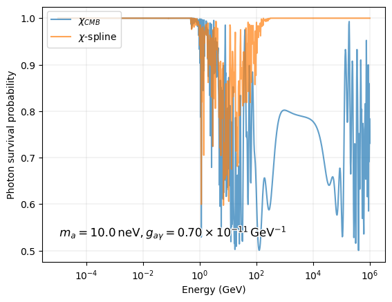
Again, including \(\chi\) lowers the highest energy at which there is strong mixing.
GMF
For the GMF:
[23]:
# GMF
ml = ModuleList(ALP(m=1., g=2.), src, pin=pin, EGeV=EGeV, seed = 0)
ml_chi = ModuleList(ALP(m=1., g=2.), src, pin=pin, EGeV=EGeV, seed = 0)
[24]:
ml.add_propagation("GMF",
                   0,
                   model='jansson12')
ml_chi.add_propagation("GMF",
                       0,
                       model='jansson12',
                       chi = chispl)
environs.py:1196 --- INFO: Using inputted chi
environs.py:1193 --- INFO: Using interpolated chi
[25]:
ml.alp.m = 1.
ml.alp.g = 3.

ml_chi.alp.m = 1.
ml_chi.alp.g = 3.
[26]:
px, py, pa = ml.run()
pgg = px + py

px_c, py_c, pa_c = ml_chi.run()
pgg_chi = px_c + py_c
   core.py: 658 --- INFO: Running Module 0: <class 'gammaALPs.base.environs.MixGMF'>
   core.py: 658 --- INFO: Running Module 0: <class 'gammaALPs.base.environs.MixGMF'>
[27]:
for p in pgg:
    plt.plot(ml.EGeV, p, label=r'$\chi_{CMB}$')

for p_c in pgg_chi:
    plt.plot(ml_chi.EGeV, p_c, label=r'$\chi$-spline')

plt.grid(True, lw = 0.2)
plt.grid(True, which = 'minor', axis = 'y', lw = 0.2)

plt.xlabel('Energy (GeV)')
plt.ylabel(r'Photon survival probability')

plt.gca().set_xscale('log')
plt.annotate(r'$m_a = {0:.1f}\,\mathrm{{neV}}, g_{{a\gamma}}'
             r' = {1:.2f} \times 10^{{-11}}\,\mathrm{{GeV}}^{{-1}}$'.format(ml.alp.m,ml.alp.g),
             xy=(0.05,0.1),
             size='large',
             xycoords='axes fraction',
             ha='left',
             **effect)
plt.legend(loc='upper left')
[27]:
<matplotlib.legend.Legend at 0x134069550>
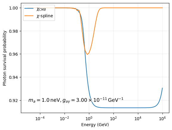
The effect is the same.
IGMF
Mixing in the IGMF is slightly different. Far from pair-produciton energies, \(\chi \propto \rho\) where \(\rho\) is the energy density of the background field. The energy density of the CMB evolves with redshift as \(\rho \propto T^4 \propto (1+z)^4\). Therefore, by default, mixing in the IGMF doesn’t use a constant value of \(\chi_{CMB}\), but rather uses \(\chi(z)=\chi_{CMB}(1+z)^4\) where \(\chi_{CMB} = 5.11\times10^{-43}\) as mentioned above and is calculated at \(z=0\).
It is also possible to manually include a spline function for \(\chi\) in the IGMF, but now the spline needs to be in energy and redshift instead of energy and distance:
[28]:
zs = np.logspace(-1,np.log10(1.5),200)
chispl_z = RBSpline(EGeV,zs,chis,kx=1,ky=1,s=0)
[29]:
# IGMF
ml = ModuleList(ALP(m=1., g=2.), src, pin=pin, EGeV=EGeV, seed = 0)
ml_chi = ModuleList(ALP(m=1., g=2.), src, pin=pin, EGeV=EGeV, seed = 0)
ml_chiz = ModuleList(ALP(m=1., g=2.), src, pin=pin, EGeV=EGeV, seed = 0)
For comparison we will also include a constant value of \(\chi_{CMB}\). Any environment will accept a single value of chi in the form of chi=np.array([chi]).
[30]:
ml.add_propagation("IGMF",
                  0, # position of module counted from the source.
                  nsim=1, # number of random B-field realizations
                  B0=1e-3,  # B field strength in micro Gauss at z = 0
                  n0=1e-7,  # normalization of electron density in cm^-3 at z = 0
                  L0=1e3, # coherence (cell) length in kpc at z = 0
                  eblmodel='dominguez', # EBL model
                  chi = np.array([chiCMB])
                  )
ml_chi.add_propagation("IGMF",
                  0, # position of module counted from the source.
                  nsim=1, # number of random B-field realizations
                  B0=1e-3,  # B field strength in micro Gauss at z = 0
                  n0=1e-7,  # normalization of electron density in cm^-3 at z = 0
                  L0=1e3, # coherence (cell) length in kpc at z = 0
                  eblmodel='dominguez', # EBL model
                 chi = chispl_z
                  )
ml_chiz.add_propagation("IGMF",
                  0, # position of module counted from the source.
                  nsim=1, # number of random B-field realizations
                  B0=1e-3,  # B field strength in micro Gauss at z = 0
                  n0=1e-7,  # normalization of electron density in cm^-3 at z = 0
                  L0=1e3, # coherence (cell) length in kpc at z = 0
                  eblmodel='dominguez' # EBL model
                  )
environs.py: 109 --- INFO: Using inputted chi
environs.py: 107 --- INFO: Using interpolated chi
[31]:
ml.alp.m = 0.1
ml.alp.g = 3.

ml_chi.alp.m = 0.1
ml_chi.alp.g = 3.

ml_chiz.alp.m = 0.1
ml_chiz.alp.g = 3.
[32]:
px, py, pa = ml.run()
pgg = px + py

px_c, py_c, pa_c = ml_chi.run()
pgg_chi = px_c + py_c

px_cz, py_cz, pa_cz = ml_chiz.run()
pgg_chiz = px_cz + py_cz
   core.py: 658 --- INFO: Running Module 0: <class 'gammaALPs.base.environs.MixIGMFCell'>
   core.py: 658 --- INFO: Running Module 0: <class 'gammaALPs.base.environs.MixIGMFCell'>
   core.py: 658 --- INFO: Running Module 0: <class 'gammaALPs.base.environs.MixIGMFCell'>
[33]:
for p in pgg:
    plt.plot(ml.EGeV, p, label=r'$\chi_{CMB}$')

for p_cz in pgg_chiz:
    plt.plot(ml_chiz.EGeV, p_cz, label=r'$\chi_{CMB} (1+z)^4$')

for p_c in pgg_chi:
    plt.plot(ml_chi.EGeV, p_c, label=r'$\chi$-spline')

plt.grid(True, lw = 0.2)
plt.grid(True, which = 'minor', axis = 'y', lw = 0.2)

plt.xlabel('Energy (GeV)')
plt.ylabel(r'Photon survival probability')

plt.gca().set_xscale('log')
plt.annotate(r'$m_a = {0:.1f}\,\mathrm{{neV}}, g_{{a\gamma}}'
             r' = {1:.2f} \times 10^{{-11}}\,\mathrm{{GeV}}^{{-1}}$'.format(ml.alp.m,ml.alp.g),
             xy=(0.05,0.1),
             size='large',
             xycoords='axes fraction',
             ha='left',
             **effect)
plt.legend()
[33]:
<matplotlib.legend.Legend at 0x137898ca0>
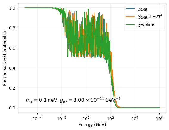
All three are different.
[ ]: